Monitoring Health Metrics Regarding Each Process on Linux

ps axo pid,ppid,rss,vsz,nlwp,cmd --sort=-rss,-vsz

Output columns:

• pid - Process ID
• ppid - Parent Process ID
• rss - Resident Set Size - physical memory
• vsz - Virtual Set Size - virtual memory
• nlwp - Number of Light Weight Processes - thread count
• cmd - Command
• --sort
• specify sorting order. Sorting syntax is [+|-]key[,[+|-]key[,...]]
• Choose a multi-letter key from the STANDARD FORMAT SPECIFIERS section.
• The "+" is optional since default direction is increasing numerical or lexicographic order.

Method to Convert Depth-First-Search From Recursion To Tail-Recursion in Scala

The earth is divided into multiple grid-like region which is represented by GeoHash. The following will start searching from a grid, whose path will be one of the (north, south, east, west) grids. The border will be distance between current grid and the starting grid.

def expand_neighbors_impl(ghCenter: GeoHash, ghCur: GeoHash, buffer: collection.mutable.Set[GeoHash]): Unit = {
    // MARK: DP: check whether it's iterated already or not
    if(buffer contains ghCur)  {
    return
    }
    buffer += ghCur

    for(ghAround <- get4GeoHashAround(ghCur))  {
    if(distanceBetweenGeohash(ghCenter, ghAround) <= radius)  {
        expand_neighbors_impl(ghCenter, ghAround, buffer)
    }
    }
}

def get4GeoHashAround(gh: GeoHash): Array[GeoHash] = {
    Array(gh.getNorthernNeighbour, gh.getSouthernNeighbour, gh.getWesternNeighbour, gh.getEasternNeighbour)
}

def distanceBetweenGeohash(gh1: GeoHash, gh2: GeoHash) = {
    haversine(gh1.getBoundingBoxCenterPoint.getLatitude, gh1.getBoundingBoxCenterPoint.getLongitude, gh2.getBoundingBoxCenterPoint.getLatitude, gh2.getBoundingBoxCenterPoint.getLongitude)
}

But the above code needs recursion, which may throw StackOverflowError. One of the way to solve it is by setting -Xss256m -Xmx4096m parameters when launching. But the more decent way to do is transfer this depth-first-search to tail-recursion:

@tailrec
def expand_neighbors_impl(ghCenter: GeoHash, toGoThrough: List[GeoHash], buffer: Set[GeoHash] = Set()): Set[GeoHash] = {
    toGoThrough.headOption match {
    case None => buffer
    case Some(ghCur) =>
        if (buffer contains ghCur) {
        expand_neighbors_impl(ghCenter, toGoThrough.tail, buffer)
        }
        else {
        val neighbors = get4GeoHashAround(ghCur).filter(distanceBetweenGeohash(ghCenter, _) <= radius)
        expand_neighbors_impl(ghCenter, neighbors ++: toGoThrough, buffer + ghCur)
        }
    }
}

def expand_neighbors(ghCenter: GeoHash, ghCur: GeoHash): Set[GeoHash] = expand_neighbors_impl(ghCenter, List(ghCur))

Resolving Maven Dependency Conflict Problem In Intellij

After deploying Spring Boot application, there's error in log complaining:

2017-04-06 10:46:14.890 ERROR 1 --- [nio-8080-exec-1] o.a.c.c.C.[.[.[/].[dispatcherServlet]    : Servlet.service() for servlet dispatcherServlet threw exception

java.lang.NoSuchMethodError: com.fasterxml.jackson.core.JsonGenerator.writeStartObject(Ljava/lang/Object;)V
        at com.fasterxml.jackson.databind.ser.std.MapSerializer.serialize(MapSerializer.java:515) ~[jackson-databind-2.8.5.jar!/:2.8.5]

This is 99% likely causing from maven dependency conflict in most scenarios.

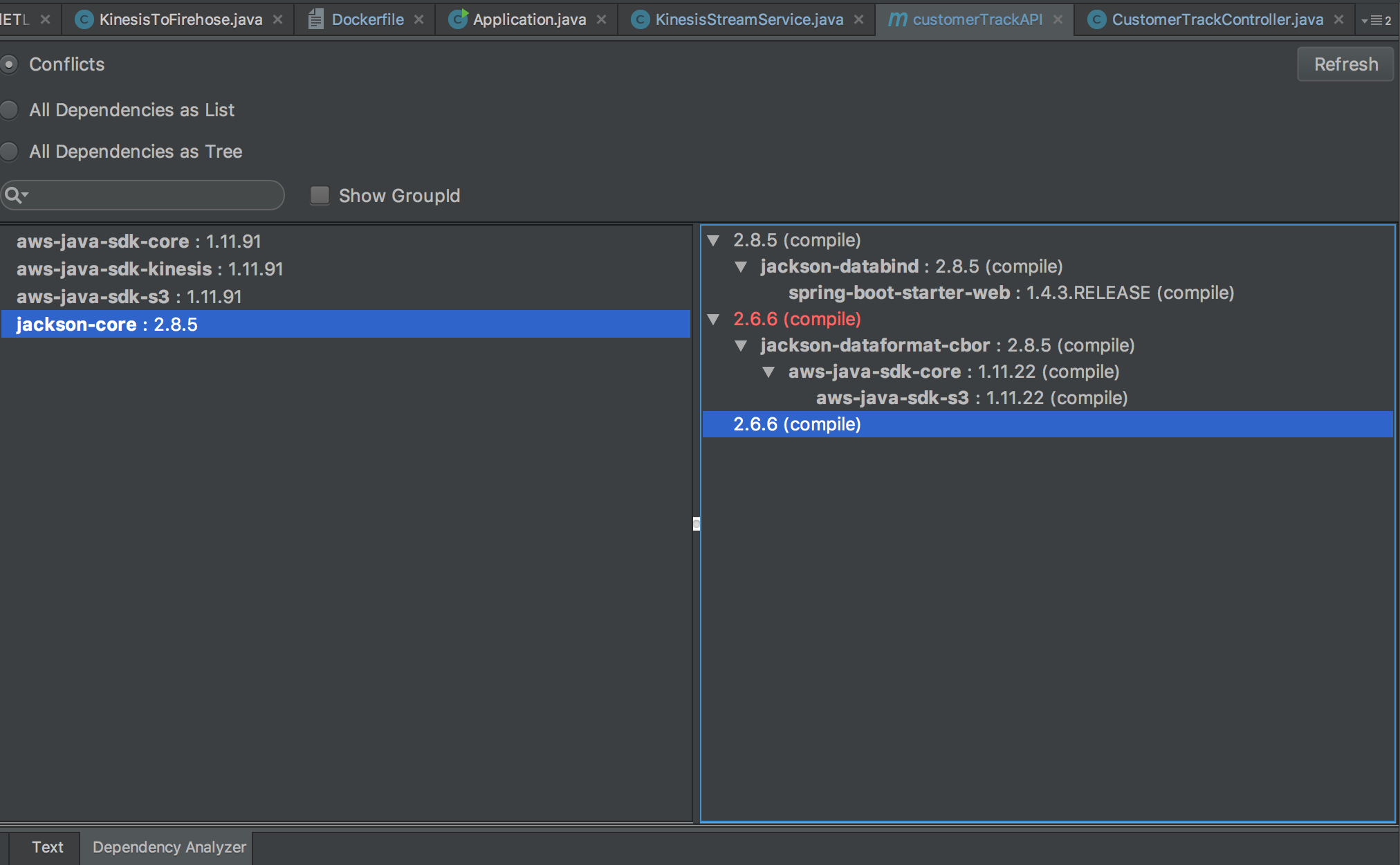
The way to solve it is always checking dependency conflict before deploying. In Intellij Idea, there's a plugin callMaven Helper, after installing, open the pom.xml file and you could find adependency analyzertab downside.

As we can see, there's two version of jackson-core packages. After going to github to check the method there, we find that 2.8.5 has methodwriteStartObject(Object forValue)whereas 2.6.6 only haswriteStartObject(). From the error above, we must exclude 2.6.6 for sure, which could be done easily independency analyzer, just right-click on the version you intend to exclude and select.

---

After deploying in docker from Elastic Beanstalk again, the error is still there, whereas if I run the jar file locally, there's no error. This is more interesting. I print thejackson-coredependency that is being used at runtime via the following java command:

System.out.println("FLAG123="+com.fasterxml.jackson.core.JsonGenerator.class.getProtectionDomain().getCodeSource().getLocation());

In this way, I could safely conclude that no error should be complained in docker deployment provided that both runtimejackson-coreis the same. And actually, my local version uses one of the other module's jar file as dependency. After excluding it from my pom.xml, all works fine again.

Spark Concept, Relationship And Tuning

1. Concept And Relationship

1.1 Static Structure

• RDD
  • resilient distributed dataset
  • a fault-tolerant collection of elements that can be operated on in parallel. (Same structure in each RDD and could change it after applying RDD operations)
  • two ways to initial RDD
    • parallelizing an existing collection in your driver program
    • referencing a dataset in an external storage system (HDFS, or any data source offering a Hadoop InputFormat)
• partition
  • Also called slice, split
  • RDD consists of multiple partitions (same data structure, could be operated in parallel)
  • Spark will run one task for each partition of the cluster. Typically you want 2-4 partitions for each CPU (vcore) in your cluster.

1.2 RDD Operations

• transformation
  • create a new dataset from an existing one
  • All transformations in Spark are lazy, in that they do not compute their results right away. Instead, they just remember the transformations applied to some base dataset.
  • The transformations are only computed when an action requires a result to be returned to the driver program.
  • By default, each transformed RDD may be recomputed each time you run an action on it. However, you may also persist an RDD in memory using the persist or cache method, in which case Spark will keep the elements around on the cluster for much faster access the next time you query it. There is also support for persisting RDDs on disk, or replicated across multiple nodes.
  • E.g. map(), filter(), groupByKey(), reduceByKey(), join(), repartition().
• action
  • return a value to the driver program after running a computation on the dataset
  • E.g. reduce(), collect(), count(), take(n), saveAsTextFile(path), foreach(func)
• narrow dependency
  • For the RDDs returned by so-called narrow transformations like map and filter, the records required to compute the records in a single partition reside in a single partition in the parent RDD. Each object is only dependent on a single object in the parent.
• wide dependency
  • transformations with wide dependencies such as groupByKey and reduceByKey. In these dependencies, the data required to compute the records in a single partition may reside in many partitions of the parent RDD. All of the tuples with the same key must end up in the same partition, processed by the same task. To satisfy these operations, Spark must execute a shuffle, which transfers data around the cluster and results in a new stage with a new set of partitions.
  • Transformations that may trigger a stage boundary typically accept a numPartitions argument that determines how many partitions to split the data into in the child stage.
  • repartition , join, cogroup, and any of the *By or *ByKey transformations can result in shuffles.

1.3 Dynamic Structure

• driver
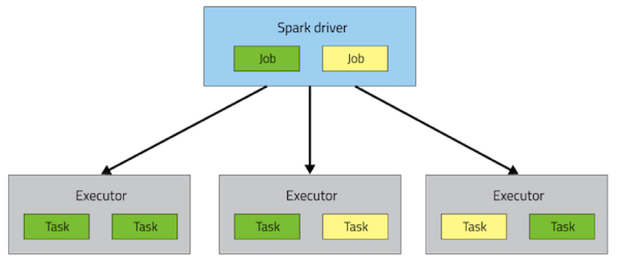
  • A Spark application consists of a single driver process and a set of executor processes scattered across nodes on the cluster
  • The driver is the process that is in charge of the high-level control flow of work that needs to be done
• job
  • At the top of the execution hierarchy are jobs. Invoking an action inside a Spark application triggers the launch of a Spark job to fulfill it
• stage
  • To decide what this job looks like, Spark examines the graph of RDDs on which that actiondepends and formulates an execution plan
  • The execution plan consists of assembling the job’s transformations into stages. A stagecorresponds to a collection of tasks that all execute the same code, each on a different subset of the data. Each stage contains a sequence of transformations that can be completed without shuffling the full data (wide dependency is the delimiter of two adjacent stages)
• node & cluster
  • node is every machine in the cluster
• task & executor
  • Spark breaks up the processing of RDD operations into tasks (one partition per task), each of which is executed by an executor
  • Executor consists of multiple tasks
  • The executor processes are responsible for executing this work, in the form of tasks, as well as for storing any data that the user chooses to cache

1.4 Miscellaneous

• Closure
  • The closure is those variables and methods which must be visible for the executor to perform its computations on the RDD (in this case foreach()). This closure is serialized and sent to each executor.
  • The variables within the closure sent to each executor are now copies and thus, when counter is referenced within the foreach function, it’s no longer the counter on the drivernode. There is still a counter in the memory of the driver node but this is no longer visible to the executors! The executors only see the copy from the serialized closure. Thus, the final value of counter will still be zero since all operations on counter were referencing the value within the serialized closure.
  • To ensure well-defined behavior in these sorts of scenarios one should use an Accumulator. Accumulators in Spark are used specifically to provide a mechanism for safely updating a variable when execution is split up across worker nodes in a cluster.

counter = 0
rdd = sc.parallelize(data)

# Wrong: Don't do this!!
def increment_counter(x):
    global counter
    counter += x
rdd.foreach(increment_counter)

print("Counter value: ", counter)

• PairRDDFunctions
  • Some RDD functions can only be applied to RDD with structure like (key, value) pairs.
  • The most common ones are distributed “shuffle” operations, such as grouping or aggregating the elements by a key.
  • E.g. groupByKey(), reduceByKey(), join().
• Shuffle
  • Spark’s mechanism for re-distributing data so that it’s grouped differently across partitions. This typically involves copying data across executors and machines, making the shuffle a complex and costly operation.
  • During computations, a single task will operate on a single partition - thus, to organize all the data for a single reduceByKey reduce task to execute, Spark needs to perform an all-to-all operation. It must read from all partitions to find all the values for all keys, and then bring together values across partitions to compute the final result for each key - this is called the shuffle.
  • Operations which can cause a shuffle:
    • repartition operations like repartition and coalesce
    • *ByKey operations (except for counting) like groupByKey and reduceByKey
    • join operations like cogroup and join
  • The Shuffle is an expensive operation since it involves disk I/O, data serialization, and network I/O. To organize data for the shuffle, Spark generates sets of tasks - map tasksto organize the data, and a set of reduce tasks to aggregate it.
• RDD Persistence
  • When you persist an RDD, each node stores any partitions of it that it computes in memory and reuses them in other actions on that dataset (or datasets derived from it). This allows future actions to be much faster (often by more than 10x). Caching is a key tool for iterative algorithms and fast interactive use.
  • Spark’s cache is fault-tolerant
    • if any partition of an RDD is lost, it will automatically be recomputed using the transformations that originally created it.
  • persist(StorageLevel.MEMORY_ONLY) = cache()
  • storage level
    • E.g. MEMORY_ONLY, MEMORY_AND_DISK, MEMORY_ONLY_SER, DISK_ONLY.
    • N.B. In Python, stored objects will always be serialized with the Pickle library, so it does not matter whether you choose a serialized level. The available storage levels in Python include MEMORY_ONLY, MEMORY_ONLY_2, MEMORY_AND_DISK, MEMORY_AND_DISK_2, DISK_ONLY, and DISK_ONLY_2.
• Shared Variables
  • Broadcast
    • to keep a read-only variable cached on each machine rather than shipping a copy of it with tasks. They can be used, for example, to give every node a copy of a large input dataset in an efficient manner.
    • broadcastVar = sc.broadcast([1, 2, 3])
  • Accumulator
    • Accumulators are variables that are only “added” to through an associative ($a+b=b+a$) and commutative ($(a+b)+c=a+(b+c)$) operation and can therefore be efficiently supported in parallel.
    • They can be used to implement counters (as in MapReduce) or sums.
    • accum = sc.accumulator(0)

---

2. Tuning

• RDD accessing method or variable in class instance
  • It is also possible to pass a reference to a method in a class instance, this requires sending the object that contains that class along with the method. Likewise, accessing fields of the outer object will reference the whole object.

    class MyClass(object):
      def func(self, s):
        return s
      def doStuff(self, rdd):
        return rdd.map(self.func)

   class MyClass(object):
      def __init__(self):
        self.field = "Hello"
      def doStuff(self, rdd):
        return rdd.map(lambda s: self.field + s)

    # To avoid this issue, the simplest way is to copy field into  
    # a local variable instead of accessing it externally.

    def doStuff(self, rdd):
      field = self.field
      return rdd.map(lambda s: field + s)

• Printing elements of RDD
  • collect() method will retrieve all elements back to driver node, which may cause OOM.
  • If only a few elements is required, take(n) method could be applied to retrieve first n elements.
• Repartition and sort (Secondary Sort)
  • repartitionAndSortWithinPartitions to efficiently sort partitions while simultaneously repartitioning
• Which storage level to choose
  • provide different trade-offs between memory usage and CPU efficiency
  • If your RDDs fit comfortably with the default storage level (MEMORY_ONLY), leave them that way. This is the most CPU-efficient option, allowing operations on the RDDs to run as fast as possible.
  • If not, try using MEMORY_ONLY_SER and selecting a fast serialization library (E.g. Kryo) to make the objects much more space-efficient, but still reasonably fast to access. (Java and Scala)
  • Don’t spill to disk unless the functions that computed your datasets are expensive, or they filter a large amount of the data. Otherwise, recomputing a partition may be as fast as reading it from disk.
  • Use the replicated storage levels if you want fast fault recovery (e.g. if using Spark to serve requests from a web application). All the storage levels provide full fault tolerance by recomputing lost data, but the replicated ones let you continue running tasks on the RDD without waiting to recompute a lost partition.
• Join optimization
  • If two datasets (Big and small in size respectively) intend to join together, the shuffle of big datasets will cause performance penalty. Thus a better way to do that is broadcast the small-in-size dataset and a map transformation can then reference the hash table to do lookups.
• Data Serialization
  • Spark can also use the Kryo library (version 2) to serialize objects more quickly. Kryo is significantly faster and more compact than Java serialization (often as much as 10x), but does not support all Serializable types and requires you to register the classes you’ll use in the program in advance for best performance. Which should always be considered firstly.
• Level of Parallelism
  • In general, 2-3 tasks/partitions per CPU core in your cluster is recommended.
  • Sometimes, you will get an OOM not because your RDDs don’t fit in memory, but because the working set of one of your tasks, such as one of the reduce tasks in groupByKey, was too large. Spark’s shuffle operations (sortByKey, groupByKey, reduceByKey, join, etc) build a hash table within each task to perform the grouping, which can often be large. The simplest fix here is to increase the level of parallelism, so that each task’s input set is smaller. Spark can efficiently support tasks as short as 200 ms, because it reuses one executor JVM across many tasks and it has a low task launching cost, so you can safely increase the level of parallelism to more than the number of cores in your clusters.
• Broadcast large variables
  • Using the broadcast functionality available in SparkContext can greatly reduce the size of each serialized task, and the cost of launching a job over a cluster. If your tasks use any large object from the driver program inside of them (e.g. a static lookup table), consider turning it into a broadcast variable. Spark prints the serialized size of each task on the master, so you can look at that to decide whether your tasks are too large; in general tasks larger than about 20 KB are probably worth optimizing.
• repartition() vs coalesce()
  • repartition() the number of partitions can be increased/decreased, but with coalesce() the number of partitions can only be decreased
  • coalesce() avoids a full shuffle. If it's known that the number is decreasing, then the executor can safely keep data on the minimum number of partitions, only moving the data off the extra nodes, onto the nodes that we kept.

Node 1 = 1,2,3
Node 2 = 4,5,6
Node 3 = 7,8,9
Node 4 = 10,11,12
Then coalesce() down to 2 partitions:

Node 1 = 1,2,3 + (10,11,12)
Node 3 = 7,8,9 + (4,5,6)
Notice that Node 1 and Node 3 did not require its original data to move.

• Avoid groupByKey()
  • Avoid groupByKey and use reduceByKey or combineByKey instead.
    • groupByKey shuffles all the data, which is slow.
    • reduceByKey shuffles only the results of sub-aggregations in each partition of the data (like the combiner in MapReduce).
    • Consequently, if we intend to do groupByKey and then reduce, we should apply reduceByKey instead.
• Avoid reduceByKey() When the input and output value types are different.
  • For example, consider writing a transformation that finds all the unique strings corresponding to each key. One way would be to use map to transform each element into a Set and then combine the Sets with reduceByKey.
  • This would result in tons of unnecessary object creation because a new set must be allocated for each record. It’s better to use aggregateByKey, which performs the map-side aggregation more efficiently
• Avoid the flatMap-join-groupBy pattern
  • When two datasets are already grouped by key and you want to join them and keep them grouped, you can just use cogroup. That avoids all the overhead associated with unpacking and repacking the groups.
• Read compressed file
  • Since comppressed file is not splittable, there will be only 1 partition for the created RDD. So we need to do repartition() after reading the file into RDD.
  • It's always better to check partition number after reading a file to make sure it could take full advantage of cluster's capacity.
• Tuning parallelism & resource (memory, vcore)
  • Reference to How-to: Tune Your Apache Spark Jobs (Part 2)

---

Reference

• https://spark.apache.org/docs/latest/programming-guide.html
• https://jaceklaskowski.gitbooks.io/mastering-apache-spark/content/spark-rdd-shuffle.html
• https://jaceklaskowski.gitbooks.io/mastering-apache-spark/content/spark-rdd-partitions.html
• http://www.edureka.co/blog/demystifying-partitioning-in-spark
• http://homepage.cs.latrobe.edu.au/zhe/ZhenHeSparkRDDAPIExamples.html
• http://blog.cloudera.com/blog/2015/03/how-to-tune-your-apache-spark-jobs-part-1/
• http://blog.cloudera.com/blog/2015/03/how-to-tune-your-apache-spark-jobs-part-2/